Atoms in Molecules (QTAIM) – Flash lesson

As far as population analysis methods goes, the Quantum Theory of Atoms in Molecules (QTAIM) a.k.a Atoms in Molecules (AIM) has become a popular option for defining atomic properties in molecular systems, however, its calculation is a bit tricky and maybe not as straightforward as Mulliken’s or NBO.

Personally I find AIM a philosophical question since, after the introduction of the molecule concept by Stanislao Cannizzaro in 1860 (although previously developed by Amadeo Avogadro who was dead at the time of the Karlsruhe congress), the questions of whether or not an atom retains its identity when bound to others? where does an atom end and the next begins? What are the connections between atoms in a molecule? are truly interesting and far deeper than we usually consider because it takes a big mental leap to think about how matter is organized to give rise to substances. Particularly I’m very interested with the concept of a Molecular Graph which in turn is concerned with the way we “draw lines” to form conceptual molecules. Perhaps in a different post we can go into the detail of the method, which is based in the Laplacian operator of the electron density, but today, I just want to collect the basic steps in getting the most basic AIM answers for any given molecule. Recently, my good friend Pezhman Zarabadi-Poor and I have used rather extensively the following procedure. We hope to have a couple of manuscripts published later on. Therefore, I’ve asked Pezhman to write a sort of guest post on how to run AIMALL, which is our selected program for the integration algorithm.

The first thing we need is a WFN or WFX file, which contains the wavefunction in a Fortran unformatted file on which the Laplacian integration is to be performed. This is achieved in Gaussian09 by incluiding the keyword output=wfn or output=wfx in the route section and adding a name for this file at the bottom line of the input file, e.g.

filename.wfn

(NOTE: WFX is an eXtended version of  WFN; particularly necessary when using pseudopotentials or ECP’s)

Analyzing this file requires the use of a third party software such as AIMALL suite of programs, of which the standard version is free of charge upon registration to their website.

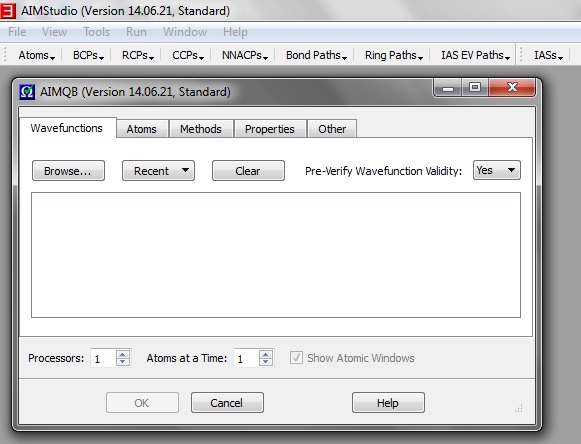
OpenAIMStudio (the accompanying graphical interface) and select the AIMQB program from the run menu as shown in figure 1.

 

Select your WFN/WFX file on which the calculation is to be run. (Figure 2)

 

You can control several options for the integration of the Laplacian of the electron density as well as other features. If your molecules are simple enough, you may go through with a successful and meaningful calculation using the default settings. After the calculation is finished, several result files are obtained. We’ll work in this tutorial only with *.mpgviz (which contains information about the molecular graph, MG) and *.sum (which contains all of  needed numerical data).

Visualization of the MG yields different kinds of critical points, such as: 1) Nuclear Attractor Critical Points (NACP); 2) Bond Critical Points (BCP); 3) Ring CP’s (RCP); and 4) Cage CP’s (CCP).

Of the above, BCP are the ones that indicate the presence of a chemical bond between two atoms, although this conclusion is not without controversy as pointed out by Foroutan-Njead in his paper: C. Foroutan-Nejad, S. Shahbazian and R. Marek, Chemistry – A European Journal, 2014, 20, 10140-10152. However, at a first approximation, BCP’s can help us to explore chemical interactions.

Now, let’s go back to visualizing those MGs (in our examples we’ve used methane and ethylene and acetylene). We open the corresponding *.mpgviz file in AIMStudio and export the image from the file menu and using the save as picture option (figure 3).

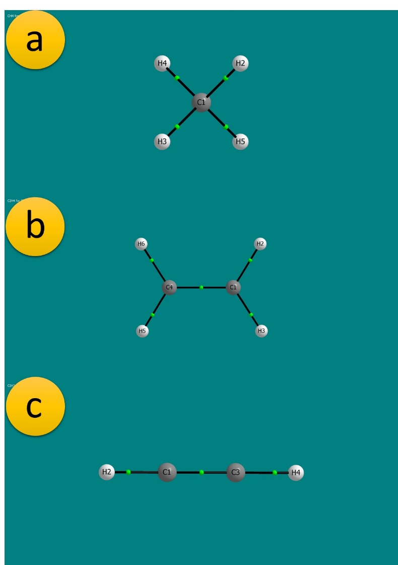
The labeled atoms are NACP’s while the green dots correspond to BCP’s. Multiplicity of a bond cannot be discerned within the MG; in order to find out whether a bond is a single, double or triple bond we have to look into the *.sum file, in which we’ll take a look at the bond orders between pairs of atoms in the section labeled “Diatomic Electron Pair Contributions and Delocalization Data” (Figure 4).

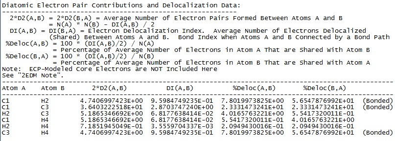
Delocalization indexes, DI’s, show the approximate number of electrons shared between two atoms. From the above examples we get the following DI(C,C) values: 1.93 for C2H4 and 2.87 for C2H2; on the other hand, DI(C,H) values are  0.98 for CH4, 0.97 in C2H4 and 0.96 in C2H2. These are our usual bond orders.

This is the first part of a crash tutorial on AIM, in my opinion this is the very basics anyone needs to get started with this interesting and widespread method. Thanks to all who asked about QTAIM, now you have your long answer.

Thanks a lot to my good friend Dr Pezhman Zarabadi-Poor for providing this contribution to the blog, we hope you all find it helpful. Please share and comment.