Orbital Contributions to Excited States

This is a guest post by our very own Gustavo “Gus” Mondragón whose work centers around the study of excited states chemistry of photosynthetic pigments.

When you’re calculating excited states (no matter the method you’re using, TD-DFT, CI-S(D), EOM-CCS(D)) the analysis of the orbital contributions to electronic transitions poses a challenge. In this post, I’m gonna guide you through the CI-singles excited states calculation and the analysis of the electronic transitions.

I’ll use adenine molecule for this post. After doing the corresponding geometry optimization by the method of your choice, you can do the excited states calculation. For this, I’ll use two methods: CI-Singles and TD-DFT.

The route section for the CI-Singles calculation looks as follows:

%chk=adenine.chk
%nprocshared=8
%mem=1Gb

#p CIS(NStates=10,singlets)/6-31G(d,p) geom=check guess=read scrf=(cpcm,solvent=water)

adenine excited states with CI-Singles method

0 1
--blank line--

I use the same geometry from the optimization step, and I request only for 10 singlet excited states. The CPCP implicit solvation model (solvent=water) is requested. If you want to do TD-DFT, the route section should look as follows:

%chk=adenine.chk
%nprocshared=8
%mem=1Gb

#p FUNCTIONAL/6-31G(d,p) TD(NStates=10,singlets) geom=check guess=read scrf=(cpcm,solvent=water)

adenine excited states with CI-Singles method

0 1
--blank line--

Where FUNCTIONAL is the DFT exchange-correlation functional of your choice. Here I strictly not recommend using B3LYP, but CAM-B3LYP is a noble choice to start.

Both calculations give to us the excited states information: excitation energy, oscillator strength (as f value), excitation wavelength and multiplicity:

Excitation energies and oscillator strengths:

 Excited State   1:      Singlet-A      6.3258 eV  196.00 nm  f=0.4830  <S**2>=0.000
      11 -> 39        -0.00130
      11 -> 42        -0.00129
      11 -> 43         0.00104
      11 -> 44        -0.00256
      11 -> 48         0.00129
      11 -> 49         0.00307
      11 -> 52        -0.00181
      11 -> 53         0.00100
      11 -> 57        -0.00167
      11 -> 59         0.00152
      11 -> 65         0.00177

The data below corresponds to all the electron transitions involved in this excited state. I have to cut all the electron transitions because there are a lot of them for all excited states. If you have done excited states calculations before, you realize that the HOMO-LUMO transition is always an important one, but not the only one to be considered. Here is when we calculate the Natural Transition Orbitals (NTO), by these orbitals we can analyze the electron transitions.

For the example, I’ll show you first the HOMO-LUMO transition in the first excited state of adenine. It appears in the long list as follows:

35 -> 36         0.65024

The 0.65024 value corresponds to the transition amplitude, but it doesn’t mean anything for excited state analysis. We must calculate the NTOs of an excited state from a new Gaussian input file, requesting from the checkpoint file we used to calculate excited states. The file looks as follows:

%Oldchk=adenine.chk
%chk=adNTO1.chk
%nproc=8
%mem=1Gb

#p SP geom=allcheck guess=(read,only) density=(Check,Transition=1) pop=(minimal,NTO,SaveNTO)

I want to say some important things right here for this last file. See that no level of theory is needed, all the calculation data is requested from the checkpoint file “adenine.chk”, and saved into the new checkpoint file “adNTO1.chk”, we must use the previous calculated density and specify the transition of interest, it means the excited state we want to analyze. As we don’t need to specify charge, multiplicity or even the comment line, this file finishes really fast.

After doing this last calculation, we use the new checkpoint file “adNTO1.chk” and we format it:

formchk -3 adNTO1.chk adNTO1.fchk

If we open this formatted checkpoint file with GaussView, chemcraft or the visualizer you want, we will see something interesting by watching he MOs diagram, as follows:

We can realize that frontier orbitals shows the same value of 0.88135, which means the real transition contribution to the first excited state. As these orbitals are contributing the most, we can plot them by using the cubegen routine:

cubegen 0 mo=homo adNTO1.fchk adHOMO.cub 0 h

This last command line is for plotting the equivalent as the HOMO orbital. If we want to plot he LUMO, just change the “homo” keyword for “lumo”, it doesn’t matter if it is written with capital letters or not.

You must realize that the Natural Transition Orbitals are quite different from Molecular Orbitals. For visual comparisson, I’ve printed also the molecular orbitals, given from the optimization and from excited states calculations, without calculating NTOs:

These are the molecular frontier orbitals, plotted with Chimera with 0.02 as the isovalue for both phase spaces:

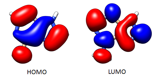
The frontier NTOs look qualitatively the same, but that’s not necessarily always the case:

If we analyze these NTOs on a hole-electron model, the HOMO refers to the hole space and the LUMO refers to the electron space.

Maybe both orbitals look the same, but both frontier orbitals are quite different between them, and these last orbitals are the ones implied on first excited state of adenine. The electron transition will be reported as follows:

If I can do a graphic summary for this topic, it will be the next one:

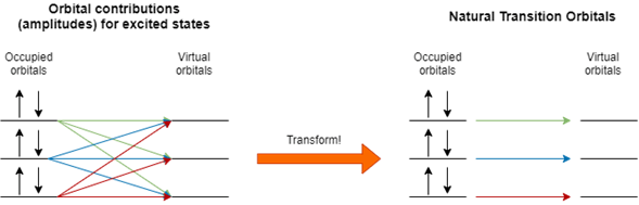
NTOs analysis is useful no matter if you calculate excited states by using CIS(D), EOM-CCS(D), TD-DFT, CASSCF, or any of the excited states method of your election. These NTOs are useful for population analysis in excited states, but these calculations require another software, MultiWFN is an open-source code that allows you to do this analysis, and another one is called TheoDORE, which we’ll cover in a later post.