
In photosynthesis research, emission spectra—particularly chlorophyll fluorescence—are not merely complementary to absorption measurements but are often more informative. While absorption spectra indicate which wavelengths are harvested, emission spectra reveal the fate of that energy, providing direct insight into its partitioning between photochemistry, heat dissipation, and fluorescence. In this way, they serve as sensitive probes of energy transfer efficiency among pigments and of the functional state of the photosystems. Characteristic emission features, including red bands (~680–690 nm) associated with Photosystem II and far-red bands (~720–740 nm) linked to Photosystem I, further enable assessment of how excitation energy is balanced across the photosynthetic apparatus.
The following is a guest post by our former member Dr. Gustavo Mondragón-Solórzano, currently working at Northeastern University on how to properly calculate absorption and emission spectra with Gaussian16.
Hey everyone! Thanks to my dear friend and colleague Joaquín for letting me share how to calculate the emission spectrum in Gaussian.
Let’s start from basics: photophysics phenomena are complex and different pathways are always possible. The two photophysical simplest phenomena I will address are absorption and emission spectroscopy.
The following diagram compares the simplified process of getting an absorption and emission spectroscopy, and the current process occurring in the Franck-Condon region. If we follow the simplified diagram we could proceed by optimizing our geometry in its ground state, and then optimize the geometry in the excited state of interest, then calculate the energy difference and get the oscillator strength as it would be a vertical excitation. However, the more realistic path is shown in the diagram on the right, where each ground state vibrational normal modes (0, 1, 2, 3) will be projected over excited state vibrational normal modes (n).
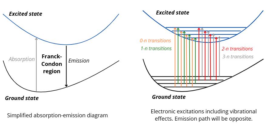
The takeaway of the diagram is that we need to calculate normal mode frequencies and include their contributions in our calculations for a more realistic absorption/emission modeling. Therefore, we need to calculate frequencies of the ground and excited state.
We need to split our workflow in two different calculations: ground state calculations and excited state calculations. I will take phenol as a practical example calculated in gas phase at the CAM-B3LYP/cc-pVDZ level of theory.
Ground state calculation is just a geometry optimization as any other geometry optimization in Gaussian. It is crucial to save the normal modes in our checkpoint file using the SaveNM keyword:
%chk=ground.chk

#p opt cam-b3lyp/cc-pvdz freq=SaveNM

Phenol ground state optimization

0 1
coords
--blank line--
We then take the final geometry from our ground state optimization as a guess for the excited state optimization and frequencies. We must also save normal modes in our excited state checkpoint file also with the same SaveNM keyword:
%oldchk=ground.chk
%chk=excited.chk

#p opt cam-b3lyp/cc-pvdz TDA(NStates=5, root=1) freq=SaveNM geom=check guess=read

Phenol excited state optimization

0 1
--blank line--
Check your final frequencies to ensure that you are on a minimum both in the ground and the excited state potential energy surfaces! You can notice that I used the keyword TDA, which solves TD-DFT equation under Tamm-Dancoff approximation, which is more efficient for excited state calculations with TD-DFT. Gaussian requires you to declare TDA to activate this approach.
Herein I showed how to call an old checkpoint file and write the calculated information in a new checkpoint file, and I’m pretty sure you have seen other posts in this blog where you call an old checkpoint file and write a new one. However, we need to call two checkpoint files at a time for a calculation considering normal modes.
Gaussian allows three different approaches to project initial and final state geometries considering normal modes. Franck-Condon, Herzberg-Teller, and the combination of both (Franck-Condon-Herzberg-Teller). Long story short, Franck-Condon factor will govern for symmetric systems, while Herzberg-Teller will govern for non symmetric systems. I will use the combination Franck-Condon-Herzberg-Teller (FCHT) approach in my calculations. Note that the keyword freq=ReadFCHT is necessary together with ReadFC to retrieve our saved normal modes. freq=ReadFCHT will also read the output after the blank line after charge and multiplicity as well. The full list of input keywords are available in ReadFCHT input in Freq | Gaussian.com.
To calculate absorption spectroscopy, the initial state is the ground state and the final state is the excited state. The input file will be:
%oldchk=excited.chk
%chk=FC.chk

#p cam-b3lyp/cc-pvdz freq=(FCHT,Read,ReadFCHT) geom=check guess=read

Phenol absorption spectrum

0 1
--blank line--
Initial=source=chk Final=Source=Calc
Transition=Absorption
Spectroscopy=OnePhotoAbsorption
--blank line--
ground.chk
--blank line--
Note this: FranckCondon, HerzbergTeller, and FCHT keywords have input lines after charge and multiplicity, if we call the geometries from the checkpoint. The line “Initial=source=Chk Final=Source=Calc” means that the initial state will be retrieved from the checkpoint file, while the final state will be retrieved from the current calculation. It will automatically take the state we set in TDA(Root=N). Transition and Spectroscopy keywords will be set as “absorption” and “OnePhotonAbsorption”, respectively. After, a blank line and then the checkpoint file name to retrieve the optimized geometry and normal modes. Similarly, emission spectrum input looks like:
%oldchk=excited.chk
%chk=FC.chk

#p CAM-B3LYP/cc-pVDZ freq=(FCHT,ReadFC,ReadFCHT) geom=check guess=read

Phenol emission spectrum

0 1

Initial=source=Calc Final=Source=Chk
Transition=Emission
Spectroscopy=OnePhotonEmission
--blank line--
ground.chk
--blank line--
Once both calculations finish, you can find the current absorption and emission spectra in the corresponding output files by looking at the specific section:
==================================================
                Final Spectrum
==================================================

 Band broadening simulated by mean of Gaussian functions with
 Half-Widths at Half-Maximum of  135.00 cm^(-1)
 Legend:
 -------
 1st col.: Energy (in cm^-1)
 2nd col.: Intensity at T=0K
 Intensity: Molar absorption coefficient (in dm^3.mol^-1.cm^-1)
 -----------------------------
    40912.2340    0.000000D+00
    40920.2340    0.000000D+00
    40928.2340    0.000000D+00
    40936.2340    0.000000D+00
…
You can directly extract the final spectrum and plot it into an excel file, or create a python code to plot it in matplotlib. We can also change half-widths at half-maximum values in the input section. We would need another line after “Spectroscopy” keyword, “Spectrum=HWHM=value”, where value variable needs to be in cm-1.
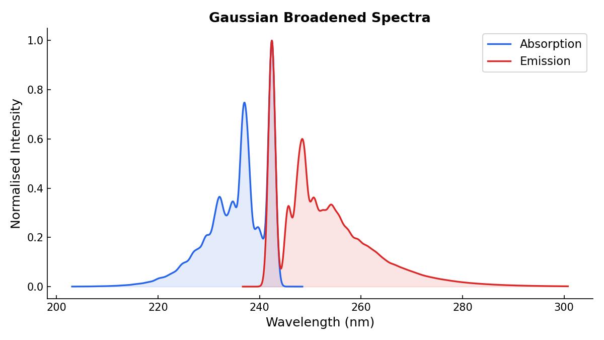
Our final absorption and emission spectra can be plotted together, showing their different vibronic transitions:
I performed a calculation with TD-DFT using TDA over the ground state optimized geometry of phenol. I plotted TD-DFT absorption spectrum using a gaussian broadening with a 0.2 eV width to show the differences of both spectra:
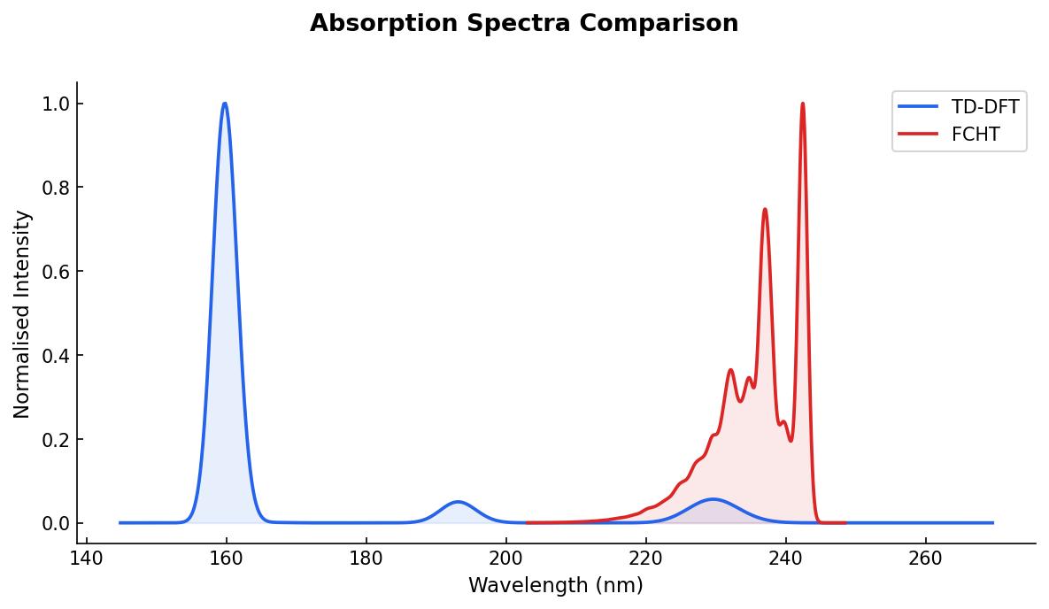
Experimentally, the maxima absorption wavelength of phenol is observed at 272 nm in methanol. The calculation is in gas phase, which means that the blue-shift is expected. However, it is noteworthy that the absorption spectrum with normal modes contributions is closer to 272 nm than the peak at 229 nm that I got with TD-DFT.
As a concluding remark I would like to say that including normal modes into the absorption and/or emission spectrum will give a more realistic modeling of the photophysical phenomenon, which you can directly compare with experimental spectra.
I hope that you find the post useful for your absorption/emission spectroscopy calculations!
