Natural Transition Orbitals (NTOs) Gaussian

The canonical molecular orbital depiction of an electronic transition is often a messy business in terms of a ‘chemical‘ interpretation of ‘which electrons‘ go from ‘which occupied orbitals‘ to ‘which virtual orbitals‘.

Natural Transition Orbitals provide a more intuitive picture of the orbitals, whether mixed or not, involved in any hole-particle excitation. This transformation is particularly useful when working with the excited states of molecules with extensively delocalized chromophores or multiple chromophoric sites. The elegance of the NTO method relies on its simplicity: separate unitary transformations are performed on the occupied and on the virtual set of orbitals in order to get a localized picture of the transition density matrix.

[1] R. L. Martin, J. Chem. Phys., 2003, DOI:10.1063/1.1558471.

In Gaussian09:
After running a TD-DFT calculation with the keyword TD(Nstates=n) (where n = number of states to be requested) we need to take that result and launch a new calculation for the NTOs but lets take it one step at a time. As an example here’s phenylalanine which was already optimized to a minimum at the B3LYP/6-31G(d,p) level of theory. If we take that geometry and launch a new calculation with the TD(Nstates=40) in the route section we obtain the UV-Vis spectra and the output looks like this (only the first three states are shown):

Excitation energies and oscillator strengths:

Excited State 1: Singlet-A 5.3875 eV 230.13 nm f=0.0015 <S**2>=0.000
42 -> 46 0.17123
42 -> 47 0.12277
43 -> 46 -0.40383
44 -> 45 0.50838
44 -> 47 0.11008
This state for optimization and/or second-order correction.
Total Energy, E(TD-HF/TD-KS) = -554.614073682
Copying the excited state density for this state as the 1-particle RhoCI density.

Excited State 2: Singlet-A 5.5137 eV 224.86 nm f=0.0138 <S**2>=0.000
41 -> 45 -0.20800
41 -> 47 0.24015
42 -> 45 0.32656
42 -> 46 0.10906
42 -> 47 -0.24401
43 -> 45 0.20598
43 -> 47 -0.14839
44 -> 45 -0.15344
44 -> 47 0.34182

Excited State 3: Singlet-A 5.9254 eV 209.24 nm f=0.0042 <S**2>=0.000
41 -> 45 0.11844
41 -> 47 -0.12539
42 -> 45 -0.10401
42 -> 47 0.16068
43 -> 45 -0.27532
43 -> 46 -0.11640
43 -> 47 0.16780
44 -> 45 -0.18555
44 -> 46 -0.29184
44 -> 47 0.43124

The oscillator strength is listed on each Excited State as “f” and it is a measure of the probability of that excitation to occur. If we look at the third one for this phenylalanine we see f=0.0042, a very low probability, but aside from that the following list shows what orbital transitions compose that excitation and with what energy, so the first line indicates a transition from orbital 41 (HOMO-3) to orbital 45 (LUMO); there are 10 such transitions composing that excitation, visualizing them all with canonical orbitals is not an intuitive picture, so lets try the NTO approach, we’re going to take excitation #10 for phenylalanine as an example just because it has a higher oscillation strength:

%chk=Excited State 10: Singlet-A 7.1048 eV 174.51 nm f=0.3651 <S**2>=0.000
41 -> 45 0.35347
41 -> 47 0.34685
42 -> 45 0.10215
42 -> 46 0.17248
42 -> 47 0.13523
43 -> 45 -0.26596
43 -> 47 -0.22995
44 -> 46 0.23277

Each set of NTOs for each transition must be calculated separately. First, copy you filename.chk file from the TD-DFT result to a new one and name it after the Nth state of interest as shown below (state 10 in this case). NOTE: In the route section, replace N with the number of the excitation of interest according to the results in filename.log. Run separately for each transition your interested in:

#chk=state10.chk

#p B3LYP/6-31G(d,p) Geom=AllCheck Guess=(Read,Only) Density=(Check,Transition=N) Pop=(Minimal,NTO,SaveNTO)

0 1
--blank line--

By requesting SaveNTO, the canonical orbitals in the state10.chk file are replaced with the NTOs for the 10th excitation, this makes it easier to plot since most visualizers just plot whatever set of orbitals they read in the chk file but if they find the canonical MOs then one would need to do some re-processing of them. This is much more straightforward.

Now we format our chk files into fchk with the formchk utility:

formchk -3 filename.chk filename.fchk
formchk -3 state10.chk state10.fchk

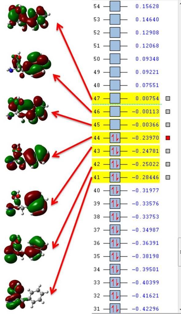
If we open filename.fchk (the file where the original TD-DFT calculation is located) with GaussView we can plot all orbitals involved in excited state number ten, those would be seven orbitals from 41 (HOMO-3) to 47 (LUMO+2) as shown in figure 1.

If we now open state10.fchk we see that the numbers at the side of the orbitals are not their energy but their occupation number particular to this state of interest, so we only need to plot those with highest occupations, in our example those are orbitals 44 and 45 (HOMO and LUMO) which have occupations = 0.81186; you may include 43 and 46 (HOMO-1 and LUMO+1, respectively) for a much more complete description (occupations = 0.18223) but we’re still dealing with 4 orbitals instead of 7.

The NTO transition 44 -> 45 is far easier to conceptualize than all the 10 combinations given in the canonical basis from the direct TD-DFT calculation. TD-DFT provides us with the correct transitions, NTOs just paint us a picture more readily available to the chemist mindset.

NOTE: for G09 revC and above, the %OldChk option is available, I haven’t personally tried it but using it to specify where the excitations are located and then write the NTOs of interest into a new chk file in the following way, thus eliminating the need of copying the original chk file for each state:

%OldChk=filename.chk
%chk=stateN.chk

NTOs are based on the Natural Hybrid orbitals vision by Löwdin and others, and it is said to be so straightforward that it has been re-discovered from time to time. Be that as it may, the NTO visualization provides a much clearer vision of the excitations occurring during a TD calculation.

Thanks for reading, stay home and stay safe during these harsh days everyone. Please share, rate and comment this and other posts.