
To calculate what the bonding properties of a molecule are in a particular excited state we can run any population analysis following the root of interest. This straightforward procedure takes two consecutive calculations since you don’t necessarily know before hand which excited state is the one of interest.
The regular Time Dependent Density Functional Theory (TD-DFT) calculation input with Gaussian 16 looks as follows (G09 works pretty much the same), let us assume we’ve already optimized the geometry of a given molecule:
%OldChk=filename.chk
%nprocshared=16
%chk=filename_ES.chk

#p TD(NStates=10,singlets) wb97xd/cc-pvtz geom=check guess=read

Title Card Required

0 1
--blank line--
This input file retrieves the geometry and wavefunction from a previous calculation from filename.chk and doesn’t write anything new into it (that is what %OldChk=filename.chk means) and creates a new checkpoint where the excited states are calculated (%chk=filename_ES.chk)
In the output you search for the transition which peeks your interest; most often than not you’ll be interested in the one with the highest oscillator strength, f. The oscillator strength is a dimensionless number that represents the ratio of the observed, integrated, absorption coefficient to that calculated for a single electron in a three-dimensional harmonic potential [Harris & Bertolucci, Symmetry and Spectroscopy]; in other words, it is related to the probability of that transition to occur, and therefore it takes values from 0.0 to 1.0 (for single photon absorption processes.)
The output of this calculation looks as follows, the value of f for every excitation is reported together with its energy and the orbital transitions which comprise it.
 Excitation energies and oscillator strengths:

 Excited State   1:      Singlet-A      3.1085 eV  398.86 nm  f=0.0043  <S**2>=0.000
      56 -> 59        -0.11230
      58 -> 59         0.69339
 This state for optimization and/or second-order correction.
 Total Energy, E(TD-HF/TD-DFT) =  -1187.56377917
 Copying the excited state density for this state as the 1-particle RhoCI density.

 Excited State   2:      Singlet-A      4.0827 eV  303.68 nm  f=0.0016  <S**2>=0.000
      52 -> 59         0.46689
      52 -> 64        -0.20488
      53 -> 59         0.19693
      54 -> 59         0.40414
      54 -> 64        -0.16261
...
...
Excited State   8:      Singlet-A      5.2345 eV  236.86 nm  f=0.8063  <S**2>=0.000
      52 -> 60         0.17162
      53 -> 59         0.47226
      53 -> 60        -0.11771
      54 -> 59        -0.27658
      54 -> 60        -0.22006
      55 -> 59         0.20496
      56 -> 59         0.15029
Now we’ve selected excited state #8 because it has the largest value of f from the lot, we use the following input to read in the geometry from the old checkpoint file and we generate a new one in case we need it for something else. The input file for doing all this looks as follows (I’ve selected as usual the Natural Bond Orbital population analysis):
%oldchk=a_ES.chk
%nprocshared=16
%chk=a_nbo.chk

#p TD(Read,Root=8) wb97xd/cc-pvtz geom=check density=current guess=read pop=NBORead

Title Card Required

0 1

$NBO BOAO BNDIDX E2PERT $END

--blank line--
The flags at the bottom request the calculation of Wiberg Bond Indexes (BNDIDX) as well as Bond Order in the Atomic Orbital basis (BOAO) and a second order perturbation theory for the electronic delocalization (E2PERT). Now we can compare the population analysis between ground and the 8th excited state; check figure 1 and notice the differences in Wiberg’s bond order for this complex made of two molecules and one Na+ cation.
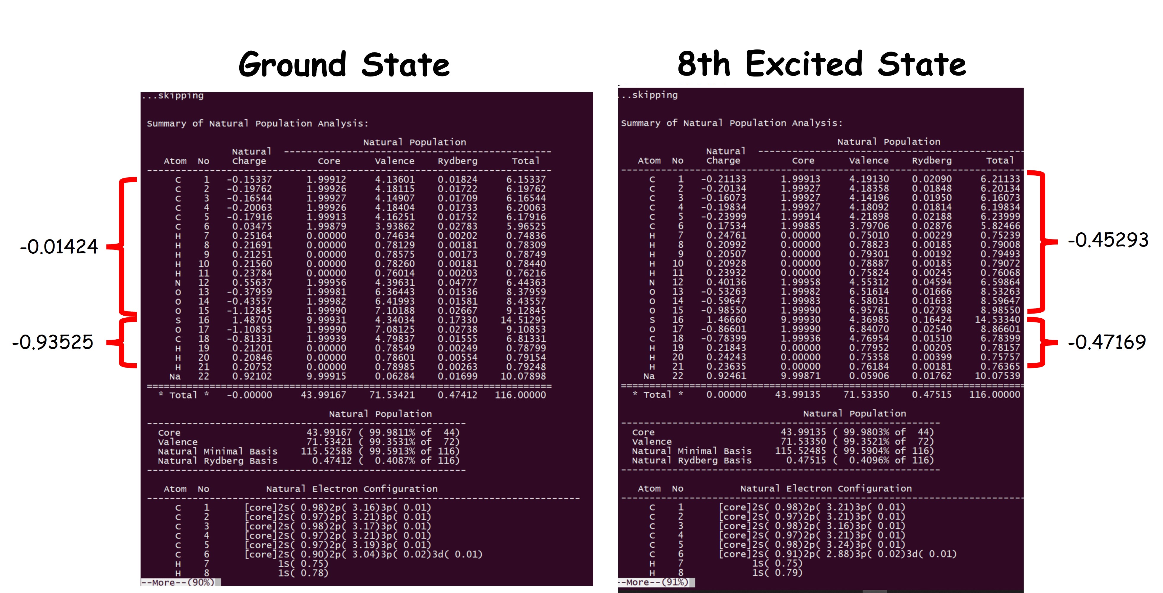
In this example we can observe that in the ground state we have a neutral and a negative molecule together with a Na+ cation, but when we analyze the population in the 8th excited state both molecules acquire a similar charge, ca. 0.46e, which means that some of the electron density has been transferred from the negative one to the neutral molecule, forming an Electron Donor-Acceptor complex (EDA) in the excited state.
This procedure can be extended to any other kind of population analysis and their derived combination, e.g. one could calculate their condensed fukui functions in the Nth excited state; but beware! These calculations yield vertical excitations, should the excited state of interest have a minimum we can first optimize the ES geometry and then perform the population analysis on said geometry; just add the opt keyword to perform both jobs in one go, but bear in mind that the NBO population analysis is performed before and after the optimization process so look for the tables and values closer to the end of the output file.
In the case of open shell systems the procedure is the same but one should be extremely careful in searching for the total population analysis since the output file contains this table for the alpha and beta populations separately as well as the added values for the total number of electrons.
